The tutorial is also hosted in GitHub.
Have you ever heard of quantum teleportation and wondered what is it exactly? Until very recently I was like you. Even if I received academic formation (including quantum mechanics) I never got past pure astonishment. For instance, once I opened a quantum information book at a public library and I was scared enough to not look further. On the other hand, popular explanations of the concept always fail to give a satisfactory description because they omit the only tool that helps us understand quantum mechanics: math.
My perspective changed completely when I encountered Nielsen and Matuschak’s Quantum Computing for the very curious fantastic essays. I encourage you to read them also.
As you will discover, most of the calculations can be reduced to simple low dimensional matrix operations. It is ideal for tinkering. Furthermore, the whole teleportation protocol can be condensed into a single diagram.
In this hands-out tutorial we will cover some of the same concepts with the help of a computer. All code below is written in Julia. Few linear algebra concepts are needed. We use the identity matrix $I_m$, the adjoint operation $A^\dagger$, the determinant, trace, kroenecker (or tensor) product, and the 2-norm.
using LinearAlgebra: I, det, tr, kron, normalize!
const ⊗ = kron
Computational quantum basis
Digital computers are able to reduce all information to zeros and ones, that is, a bit may be one of the set ${0, 1}$. The measurement of a single bit is described by a probability distribution on the space of possible bits $p: {0,1} \to [0,1]$. On the other hand, quantum bits belong to a two-dimensional complex vector space $\mathbb{C}^2$. Measurements give also a probability but draw from a larger space $\rho_p: \mathbb{C}^2 \to [0,1]$.
Now you might ask how to move data stored in bits to qubits. It turns out that you can map every classical probability distribution to a quantum probability distribution. The resulting distribution is called a density operator, $\rho_p$. If we think of each element of the bitset ${0,1}$ as a $2 \times 1$ basis vector, both form an orthonormal basis that spans $\mathbb{C}^2$.
- $|0\rangle = [1, 0]^T$ is a column vector representing the classical bit 0
- $|1\rangle = [0, 1]^T$ is a column vector representing the classical bit 1
Column vectors are represented with the bar and right bracket, e.g. $|v\rangle$, following in Dirac notation. Those two special vectors will be assigned in code to unicode characters that ressemble $0$ and $1$.
𝟎 = [1, 0] # ≡ $|0\rangle$; typeset with \bfzero
𝟏 = [0, 1] # ≡ $|1\rangle$; typeset with \bfone
The density operator is the $2 \times 2$ matrix with the classical probabilities arranged along its diagonal, the rest zeros. If we have a classical bit 0 (probability $p=1$ to have $|0\rangle$ and $p=0$ to have $|1\rangle$), then the density operator is
ρ𝟎 = [1 0;
      0 0]
Other way to map classical to quantum probabilities is using the outer product $\rho_p = \sum_i p_i |\psi_i\rangle \langle\psi_i|$
@assert ρ𝟎 ≈ 1𝟎*𝟎' + 0𝟏*𝟏' # 𝟎 has p=1, and 𝟏 has p=0 probability
The vector with left angle and bar is a row vector that is the adjoint of the corresponding column vector.
The same probability distribution can be arranged as a vector if we had chosen the tensor product instead of the outer product. Instead of a $2 \times 2$ matrix we have a $4 \times 1$ vector. Technically, a vector space like $\mathbb{C}^2$ is isomorphic to $\mathbb{C} \otimes \mathbb{C}$.
@assert vec(ρ𝟎) ≈ 1𝟎 ⊗ 𝟎 + 0𝟏 ⊗ 𝟏
A general qubit
A general qubit $|\psi\rangle = \alpha |0\rangle + \beta |1\rangle \in \mathbb{C}^2$ is described as a linear combination of the basis vectors and it must satisfy the normalization condition $|\alpha|^2 + |\beta|^2 = 1$.
α = 0.6
β = 0.8
@assert α^2 + β^2 ≈ 1 # normalization contraint (here for α, β ∈ ℝ)
ψ = α*𝟎 + β*𝟏
@assert ψ ≈ [α, β]
@assert ψ'*ψ ≈ 1 # ⟨ψ|ψ⟩ = 1 (normalization again)
Quantum gates
Once we have transformed our information to qubits we need to manipulate them to achieve our goal. Those operations are realized with gates that are analogous to classical circuit gates.
Pauli $\sigma_x$ gate: X == NOT == ---[ X ]---
X = [0 1; 1 0]
@assert X*𝟎 ≈ 𝟏
@assert X*𝟏 ≈ 𝟎
# By the linearity of matrix multiplication it follows that the matrix acts the
# same way as the X on all input states, and so they are the same operation.
@assert X*X' ≈ I(2) # this is a proof of unitariness
X*ψ
2-element Array{Float64,1}:
 0.8
 0.6
Hadamard gate: H == ---[ H ]---
A Hadamard gate converts a classical bit into a general qubit.
H = [1 1; 1 -1]./√2
@assert H*𝟎 ≈ [1, 1]./√2 # kinda bonding state
@assert H*𝟏 ≈ [1,-1]./√2 # kinda antibonding state
# By the linearity of matrix multiplication it follows that the matrix acts the
# same way as the Hadamard on all input states, and so they are the same
# operation.
@assert H^2 ≈ I(2) # H is idempotent
@assert H*H' ≈ I(2) # this is a proof of unitariness
@assert abs(det(H)) ≈ 1 # conservation of particles
Not every matrix is a gate, for instance
J = [1 1; 1 1]./√2
@assert (J*J' ≈ I(2)) == false
H X ψ == —[ X ]—[ H ]—
Measurement: ---| m )===
In colloquial terms, measurements can be performed by “casting the shadow” of the qubit state at a place where we can look, that is, our computational quantum basis. The probability of $|u\rangle$ being $|0\rangle$ is $\langle u|0\rangle\langle 0|u\rangle = |\langle 0|u\rangle|^2$ or $Tr(\rho_u |0\rangle\langle 0|)$ where $\rho_u$ is the density operator $|u\rangle\langle u|$.
measure(ψ, verbose=false) = begin
   p𝟎 = tr(ψ*ψ' * 𝟎*𝟎') # ≡ ⟨ψ|0⟩⟨0|ψ⟩ resol. ident
   p𝟏 = tr(ψ*ψ' * 𝟏*𝟏') # ≡ ⟨ψ|1⟩⟨1|ψ⟩ resol. ident
   if verbose
      println("m = 0 with probability $p𝟎")
      println("m = 1 with probability $p𝟏")
   end
   [p𝟎, p𝟏]
end
# _ψ2 ---[ H ]---[ m )===
_ψ = rand([𝟎,𝟏])
_ψ2 = H*_ψ # Input state is either (|0⟩ + |1⟩)/√2 or (|0⟩ - |1⟩)/√2
H*_ψ2 |> measure
2-element Array{Float64,1}:
 0.0
 0.9999999999999996
The state measured is the same as the initial one. That is a consequence of $H$ being idempotent.
Pauli $\sigma_y$ gate: Y == ---[ Y ]---
Y = [0 -im; im 0]
@assert Y*Y' ≈ I(2)
Pauli $\sigma_z$ gate: Z == ---[ Z ]---
Z = [1 0; 0 -1]
@assert Z*Z' ≈ I(2)
General rotation gate
θ = π/2
R = [cos(θ) -sin(θ); sin(θ) cos(θ)]
2×2 Array{Float64,2}:
 6.12323e-17  -1.0
 1.0           6.12323e-17
@assert R*R' ≈ I(2)
Rx(θ) = cos(θ/2)*I(2) - im * sin(θ/2)*X
Ry(θ) = cos(θ/2)*I(2) - im * sin(θ/2)*Y
Rz(θ) = cos(θ/2)*I(2) - im * sin(θ/2)*Z
Multi-qubit states
Here again, we can find an analogy with the classical world if we think that we are passing from sets to vector spaces. Whereas classical state spaces are combined with the cartesian product, such as ${0,1} \times {0,1}$, quantum state spaces are combined with the tensor product, $\mathbb{C}^2 ⊗ \mathbb{C}^2$. The classical probability $p: {0,1} \times {0,1} \to [0,1]$ on the combined set is a joint probability (the probability of both having 0 in the first and 0 in the second bit, for example). The corresponding density operator is also a joint probability in their tensor product space $\rho_p: \mathbb{C}^2 \otimes \mathbb{C}^2 \cong \mathbb{C}^4 \to [0,1]$.
𝟎𝟎 = 𝟎 ⊗ 𝟎
𝟎𝟏 = 𝟎 ⊗ 𝟏
𝟏𝟎 = 𝟏 ⊗ 𝟎
𝟏𝟏 = 𝟏 ⊗ 𝟏
γ = 0.8
δ = 0.6
ϕ = γ*𝟎 + δ*𝟏
2-element Array{Float64,1}:
 0.8
 0.6
More generally, if we have single-qubit states ψ and ϕ, then the combined state when the two qubits are put together is just:
ξ = ψ ⊗ ϕ
@assert ξ ≈ [ψ[1]*ϕ[1], ψ[1]*ϕ[2], ψ[2]*ϕ[1], ψ[2]*ϕ[2]]
Multi-qubit gates
Take the form $G_1 \otimes G_2 \otimes \cdots$.
Controlled-NOT gate (CNOT)
  x ---⋅---
       |
  y ---⊕---
  x is the control qubit
  y is the target qubit
  |x, y ⊕ x⟩ for short
CNOT = [1 0 0 0;
        0 1 0 0;
        0 0 0 1;
        0 0 1 0]
# Also
@assert CNOT ≈ cat(I(2), X, dims=(1,2)) #|> Matrix
@assert CNOT ≈ 𝟎*𝟎' ⊗ I(2) + 𝟏*𝟏' ⊗ X
@assert CNOT*𝟎𝟎 ≈ 𝟎𝟎
@assert CNOT*𝟎𝟏 ≈ 𝟎𝟏
@assert CNOT*𝟏𝟎 ≈ 𝟏𝟏
@assert CNOT*𝟏𝟏 ≈ 𝟏𝟎
# Apply H to first qubit in a 2d space
H₁ = H ⊗ I(2)
# Apply H to second qubit in a 2d space
H₂ = I(2) ⊗ H
4×4 Array{Float64,2}:
 0.707107   0.707107  0.0        0.0
 0.707107  -0.707107  0.0        0.0
 0.0        0.0       0.707107   0.707107
 0.0        0.0       0.707107  -0.707107
CNOT*H₁*𝟎𝟎
4-element Array{Float64,1}:
 0.7071067811865475
 0.0
 0.0
 0.7071067811865475
Beware, CNOT can change the control qubit!
# |+-⟩
pm = H*𝟎 ⊗ H*𝟏
# |--⟩
mm = H*𝟏 ⊗ H*𝟏
|0⟩ ---[ H ]--- |+⟩---⋅--- |-⟩
                      |
|1⟩ ---[ H ]--- |-⟩---⊕--- |-⟩
@assert CNOT*pm ≈ mm
Toffoli gate CCNOT
Replaces the classical AND gate
#CCNOT = cat(I(6), [0 1; 1 0], dims=(1,2)) |> Matrix
CCNOT = cat(I(4), CNOT, dims=(1,2)) |> Matrix
8×8 Array{Int64,2}:
 1  0  0  0  0  0  0  0
 0  1  0  0  0  0  0  0
 0  0  1  0  0  0  0  0
 0  0  0  1  0  0  0  0
 0  0  0  0  1  0  0  0
 0  0  0  0  0  1  0  0
 0  0  0  0  0  0  0  1
 0  0  0  0  0  0  1  0
Global phase factor
θ = rand() # any real number
0.24805413652694797
G(θ) = ℯ^(im*θ) * I(2) # global phase factor ℯ^(iθ)
if typeof(θ) <: Real
   @assert G(θ)*G(θ)' ≈ I(2)
   @info "A matrix changing the global phase factor is unitary."
end
┌ Info: A matrix changing the global phase factor is unitary.
@info "Changing the phase does not affect the measurement."
@assert G(rand())*𝟎 |> measure ≈ measure(𝟎)
┌ Info: Changing the phase does not affect the measurement.
Other gates
S = [ 1 0; 0 im]
T = [ 1 0; 0 ℯ^(im*π/4)]
#Y = [ 0 -im; im 0]
#Z = [ 1 0; 0 -1]
2×2 Array{Complex{Float64},2}:
 1.0+0.0im       0.0+0.0im
 0.0+0.0im  0.707107+0.707107im
If you were able to follow me you are ready to understand quantum teleportation.
Quantum teleportation
Alice and Bob can share beforehand a special entangled two-qubit
|0⟩ ---[ H ]---⋅---
               |
               |    (|00⟩ + |11⟩)/√2
               |
|0⟩ -----------⊕---
ebit = CNOT*H₁*𝟎𝟎 # entangled bit -> shared
4-element Array{Float64,1}:
 0.7071067811865475
 0.0
 0.0
 0.7071067811865475
Alice takes the upper qubit and Bob the lower qubit. Then, they can separate.
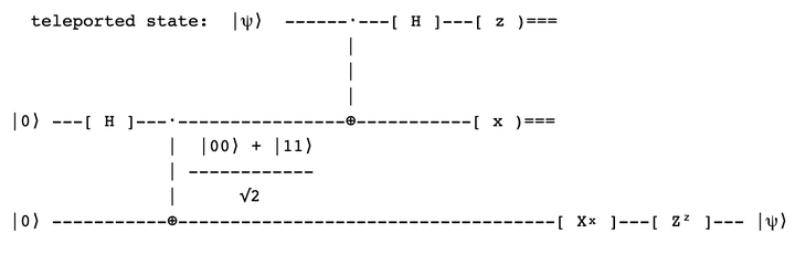
That is the first stage of the protocol depicted below
         teleported state:  |ψ⟩  ------⋅---[ H ]---[ z )===
                                       |
                                       |
                                       |
       |0⟩ ---[ H ]---⋅----------------⊕-----------[ x )===
                      |  |00⟩ + |11⟩
                      | ------------
                      |      √2
       |0⟩ -----------⊕------------------------------------[ Xˣ ]---[ Zᶻ ]--- |ψ⟩
It is a very succint way of condensing an otherwise unexpeced phenomenom.
Given the moment, Alice will desire to deliver Bob some important piece of information encoded as a qubit.
# The state ψ Alice wants to teleport
α = rand(Complex{Float64})
β = sqrt(1 - α*conj(α)) # |α|² + |β|² = 1
@assert α*conj(α) + β*conj(β) ≈ 1 "State not properly normalized. Try with other (α,β)"
ψ = α*𝟎 + β*𝟏 # ∈ ℂ² ≝ ℂ ⊗ ℂ ; ρψ = ψ*ψ' ∈ ℂ ⊗ ℂ
_ψ = ψ # we can do this only in a classic circuit (debugging purposes)
2-element Array{Complex{Float64},1}:
    0.75190393025605 + 0.5381299416639849im
 0.38086302728175303 + 0.0im
She applies a conditional-NOT to the entangled qubit based on the state to be teleported. Thus, both are entangled. Next, applies a Hadamard matrix to the state to be teleported.
s = ψ ⊗ ebit;
gate1 = CNOT ⊗ I(2)
gate2 = H ⊗ I(4);
ψ = gate2*gate1*s;
Alice measures first two bits, posibilities are 00, 01, 10, and 11
P𝟎𝟎 = 𝟎𝟎*𝟎𝟎' ⊗ I(2) # projections
P𝟎𝟏 = 𝟎𝟏*𝟎𝟏' ⊗ I(2)
P𝟏𝟎 = 𝟏𝟎*𝟏𝟎' ⊗ I(2)
P𝟏𝟏 = 𝟏𝟏*𝟏𝟏' ⊗ I(2);
ρψ = ψ*ψ' # density operator
p𝟎𝟎 = tr(ρψ * P𝟎𝟎) |> real # probabilities
p𝟎𝟏 = tr(ρψ * P𝟎𝟏) |> real
p𝟏𝟎 = tr(ρψ * P𝟏𝟎) |> real
p𝟏𝟏 = tr(ρψ * P𝟏𝟏) |> real;
@info "  The probability of |𝟎𝟎⟩ is $p𝟎𝟎"
@info "  The probability of |𝟎𝟏⟩ is $p𝟎𝟏"
@info "  The probability of |𝟏𝟎⟩ is $p𝟏𝟎"
@info "  The probability of |𝟏𝟏⟩ is $p𝟏𝟏"
┌ Info:   The probability of |𝟎𝟎⟩ is 0.2499999999999999
┌ Info:   The probability of |𝟎𝟏⟩ is 0.2499999999999999
┌ Info:   The probability of |𝟏𝟎⟩ is 0.2499999999999999
┌ Info:   The probability of |𝟏𝟏⟩ is 0.2499999999999999
All outcomes have the same chance of appearing.
icollapsed = argmax([p𝟎𝟎, p𝟎𝟏, p𝟏𝟎, p𝟏𝟏])
icollapsed = rand(1:4) # to avoid taking always the first
Pcollapsed = [P𝟎𝟎, P𝟎𝟏, P𝟏𝟎, P𝟏𝟏][icollapsed];
x = (icollapsed == 2 || icollapsed == 4) |> Int
z = (icollapsed == 3 || icollapsed == 4) |> Int
@info "  Alice measured x = $x and z = $z"
@info "  Alice qubits collapsed to $(["|𝟎𝟎⟩", "|𝟎𝟏⟩", "|𝟏𝟎⟩", "|𝟏𝟏⟩"][icollapsed])"
┌ Info:   Alice measured x = 1 and z = 0
┌ Info:   Alice qubits collapsed to |𝟎𝟏⟩
The resulting two classical bits are shared to Bob, who uses them to process his entangled bit.
range = 2icollapsed-1:2icollapsed
ψ = normalize!(Pcollapsed*ψ)[range] # state after measurement of 𝟎𝟎
ψ = Z^z * X^x * ψ # Bob uses Alice classical bits x and z
@assert _ψ ≈ ψ "Teleported state has been corrupted"
@info "  Teleported |ψ⟩ = ($(ψ[1])) |𝟎⟩ + ($(ψ[2])) |𝟏⟩ !!"
┌ Info: Teleported |ψ⟩ = (0.75190393025605 + 0.5381299416639849im) |𝟎⟩ + (0.3808630272817531 + 0.0im) |𝟏⟩ !!
This is awesome! We have teleported a vast amount information just moving two bits. It is like seeing a sportsman pulling a truck with his beard!
Teleportation technology
While this may seem just a theoretical result, recent experiments suggest that an internet based on quantum technology could be feasible. A collaborative team of researchers teleported qubits (as photon states) over a 44 km fiber optic with a fidelity above 90%. The results have been published in PRX Quantum.